Google Sheets has a great list of features focusing on productivity, Google spreadsheets have numerous formula bars for making data easy and beautiful. If you know the Google sheets formulas, then you can easily make heavy data more crisp and understandable. Nowadays more businesses are using Google Spreadsheets and making decisions by understanding their data, the usage of Google Drive Sheets has expanded enormously.
So if you want to be a pro in using Google Sheets, it’s important to understand the main backbone of this tool and the use of the Google Sheet formula. However, you can also use work in Google Drive sheets but this time consuming and not recommended for big data.
How to Use Formula in Google Sheets
- Select the specific cell you want to insert the formula in. (If you want the formula for the entire row, these may be the first or second row in a column.)
- Type the equal (=) sign.
- Type your formula. Depending on the data, Sheets may give you the formula list and/or range for you.
Best Google Sheets Formulas
1. COUNTIF
If you’ve been manually counting cells in sheets every time, Then the COUNTIF formula can complete your work easily in a single line of code.
Formula: =COUNTIF(range, criteria)
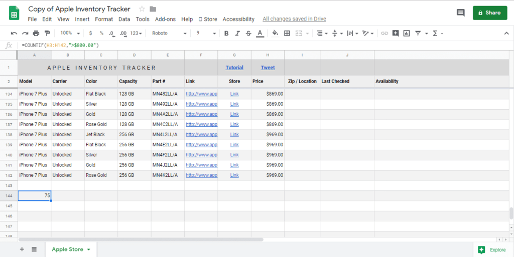
For example, if I have lots of products on my sheet and I want to count how many product’s prices are above $800 – I’d enter:
=COUNTIF(H3:H142,”>$800.00″)
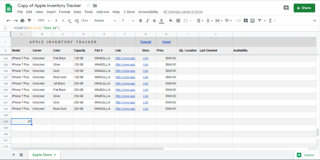
Or maybe I want to see how many product prices are equal to $969.
=COUNTIF(H3:H142,”$969.00″)
2. IFERROR
Every data is not 100% accurate all the time. IFERROR is helpful in dealing with cell errors.
You can understand by this easy example If there is an error such as #DIV/0! in Google Spreadsheet and you want to change it. So here you can fill empty data with specific text. Hence, you can use this formula to do this.
=IFERROR(value, [value_if_error])
The first parameter, value, refers to the value to return if the value is not an error.
The second parameter, value_if_error, refers to the value the function returns if the value is an error. This is left blank by default.
3. Update Current Date using TODAY() Formula
If you want to update Google Sheet’s date automatically, this formula can help you
Happily, this is the most simple Google Sheets trick available on this list.
= TODAY()
Image insert
You can also use this formula for making a report’s date range. You can do this by typing a formula like this.
Your start date would be like this =TODAY() – 7
End date would be today =TODAY()
4. TEXT() to Convert Numbers into Currency Format
Using this formula you can easily convert text data into a beautiful format. However, you can also use this formula for modifying another format. You can use it this way:
- Changing a number to have more decimal places is another format
- Changing a date string into a MM/DD format
So if you want to convert numbers into currency, here is an easy formula.
Assuming your first cell is C3, you’d use the formula =TEXT(C3,”$0.00″)
5. Divide Data into Multiple Cells Using SPLIT()
The split formula is very useful when you are dealing with different URLs. you can split data from a single cell to multiple cells.
This formula is very helpful for splitting text. You can simply split text without consuming lots of time.
Here’s the formula: =SPLIT(Text, Delimiter)
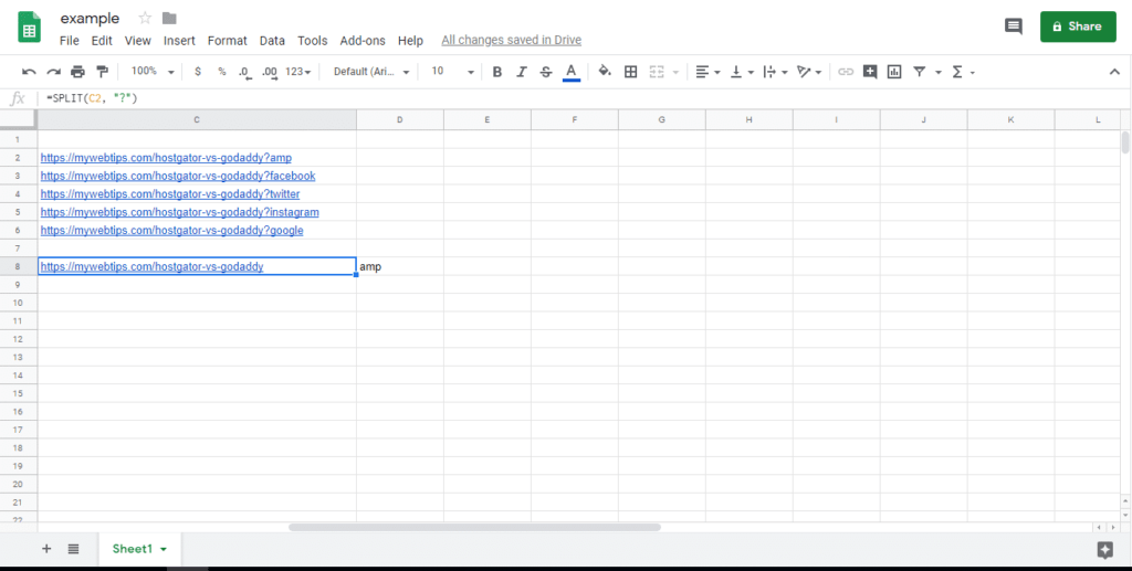
Let’s remove the different versions of the URL from the list.
=SPLIT(C2, “?”)
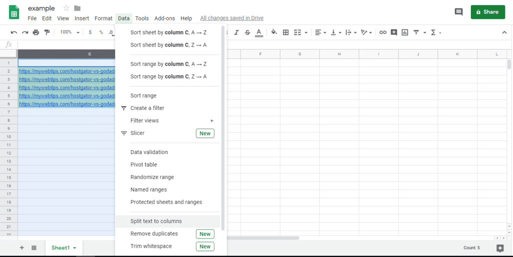
Alternatively, you can use Google Sheet’s “Split text to columns” feature from the formula bar. Select the range of data you want to split, then go to “Data” > “Split text to columns.”
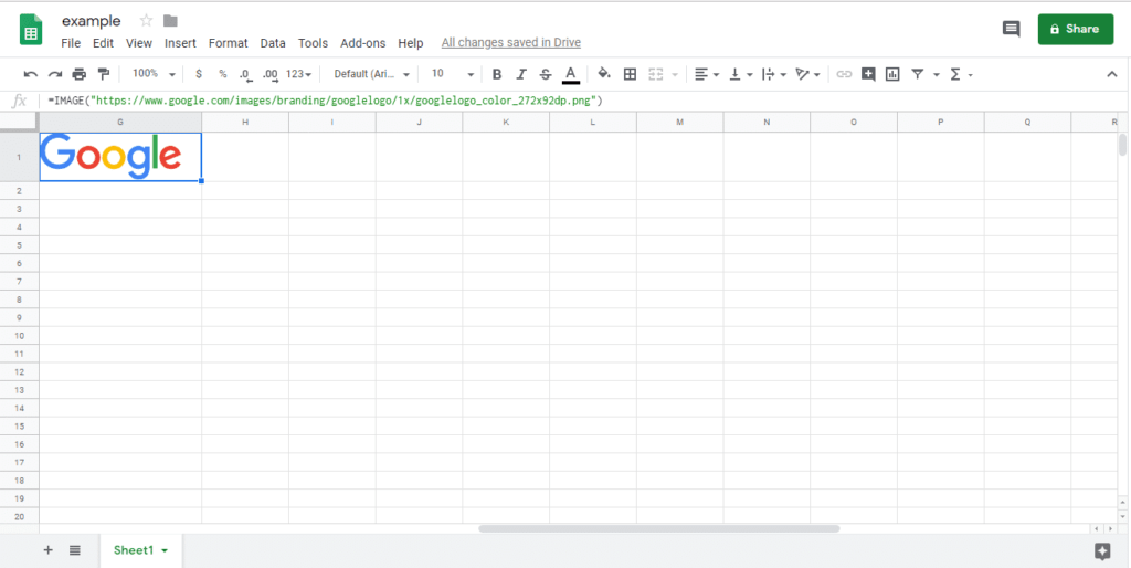
6. Insert Image by Using Image()
With this formula, you can insert an image in any column.
Formula: =IMAGE(url, [height], [width])
=IMAGE(“https://www.google.com/images/branding/googlelogo/1x/googlelogo_color_272x92dp.png“)
7. Import Data From Any Website Using IMPORTXML()
This is an amazing formula. You can easily scrape basic data from any website.
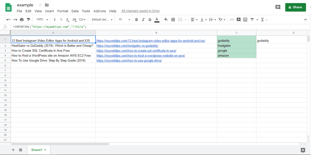
A copy-paste work can take you forever to do this! Instead, use the formula ImportXML to import information from any of the XML fields of the website to separate cells.
=IMPORTXML(url, xpath_query)
Example: If you want to import all the post titles on this URL – https://147-185-239-16.cloud-xip.com/, from its structured data, use this formula like – =IMPORTXML(“https://147-185-239-16.cloud-xip.com/”, “//h2/a”).
Here is the result of this formula.
8. Google Sheets VLOOKUP() Function to Find Value in a String
This Google Spreadsheets shortcut allows you to find whether a value exists in a string. it helps you to look up specific information located in a table or database.
=VLOOKUP(search_key, range, index, is_sorted)
First, the search_key refers to the value you want to search for.
Alongside, the range belongs to a number of columns and rows that should be included in the search.
The index refers to the column index of the value to be returned, with the first column in the range being numbered 1. Remember that if you type an index that isn’t between 1 and the number of columns in the range, “#VALUE!” will be returned.
Wrapping Up
So, those were the best and the most simple formula you can to learn if you’ve just started working on a spreadsheet!. if you think any good formula is missing in this list, then write in the comment below and we will update this post.
Here is the link of pdf file
you can also learn how google sheets work on google drive.
